3 releases (breaking)
Uses new Rust 2024
| new 0.47.0 | Jun 2, 2026 |
|---|---|
| 0.44.0 | May 29, 2026 |
| 0.43.0+000 | May 26, 2026 |
#6 in #colormap
1.5MB
37K
SLoC
ccalc
A fast terminal calculator with Octave/MATLAB syntax and script support — one binary, no runtime.
Current version: 0.48.0 — see CHANGELOG for history.
Why ccalc?
Octave is hundreds of megabytes. Python requires a runtime. ccalc is a single self-contained binary that starts instantly and works anywhere: interactive sessions, shell scripts, CI pipelines, Docker containers.
It speaks Octave/MATLAB syntax — familiar to engineers and scientists — without requiring a full language installation.
| Who | Typical use |
|---|---|
| Embedded / systems engineer | Arithmetic, hex/bin conversions, bit masks |
| DevOps / SRE | Quick calculations in scripts and pipelines |
| Scientist / student | Interactive session with variables and math functions |
| MATLAB / Octave user | Familiar syntax, no heavy installation |
Installation
git clone https://github.com/holgertkey/ccalc
cd ccalc
cargo build --release
The binary is placed at target/release/ccalc. Copy it anywhere on your PATH.
Usage
ccalc [OPTIONS]           start interactive REPL
ccalc "EXPR"              evaluate expression and print result
ccalc script.m            run a script file
echo "EXPR" | ccalc       pipe mode — silent, result only
ccalc < formulas.txt      read expressions from file
| Option | Description |
|---|---|
-h, --help |
Show help |
-v, --version |
Show version |
Modes
Interactive REPL
Run without arguments:
$ ccalc
[ 0 ]:
Single expression
Pass an expression as a command-line argument:
$ ccalc "2 ^ 32"
4294967296

$ ccalc "sqrt(144)"
12
Script file
Pass a script file as an argument — any file that exists on disk:
$ ccalc script.m
$ ccalc script.calc
$ ccalc examples/mortgage.calc
Pipe / non-interactive mode
When stdin is not a terminal, ccalc runs silently — no prompt, one result per line. ans carries over across lines, so you can chain calculations:
$ echo "sin(pi / 6)" | ccalc
0.5

$ printf "10\n+ 5\n* 2" | ccalc
10
15
30

$ ccalc < formulas.txt
All commands work in script/pipe mode: exit/quit stop processing, who/clear/ws/wl/save/load manage variables, format controls number display, hex/dec/bin/oct/base control number base. cls is ignored.
How it works
The prompt shows ans — the result of the last expression. Every new expression updates it. Expressions that start with an operator automatically use ans as the left-hand operand (partial expressions):
[ 0 ]: 100
[ 100 ]: / 4
[ 25 ]: + 5
[ 30 ]: ^ 2
[ 900 ]:
Arithmetic
Operators
| Operator | Description | Precedence |
|---|---|---|
^ |
Power (right-associative) | highest |
* / |
Multiply, divide | medium |
+ - |
Add, subtract | lowest |
[ 0 ]: 2 + 3 * 4
[ 14 ]:

[ 0 ]: 2 ^ 3 ^ 2
[ 512 ]:               (right-associative: 2^(3^2) = 2^9)
Grouping
[ 0 ]: (2 + 3) * 4
[ 20 ]:
Unary minus
[ 0 ]: -5
[ -5 ]:

[ 0 ]: -(3 + 2)
[ -5 ]:
Ergonomics
Implicit multiplication
A number or closing parenthesis immediately before ( multiplies without an explicit *:
[ 0 ]: 2(3 + 1)
[ 8 ]:

[ 0 ]: (2 + 1)(4 - 1)
[ 9 ]:
Constants
| Name | Value |
|---|---|
pi |
3.14159265358979... |
e |
2.71828182845904... |
nan |
Not-a-Number (IEEE 754 NaN) |
inf |
Positive infinity |
i, j |
Imaginary unit 0 + 1i (can be reassigned) |
ans |
Result of the last expression |
ans is the implicit accumulator — it is updated after every expression and can be used anywhere in an expression:
[ 9 ]: ans * 2 + 1
[ 19 ]:

[ 25 ]: sqrt(ans)
[ 5 ]:
Math functions
If called with empty parentheses, ans is used as the argument.
One-argument
| Function | Description |
|---|---|
sqrt(x) |
Square root |
abs(x) |
Absolute value |
floor(x) |
Round down to integer |
ceil(x) |
Round up to integer |
round(x) |
Round to nearest integer |
sign(x) |
Sign: −1, 0, or 1 |
log(x) |
Base-10 logarithm |
ln(x) |
Natural logarithm (base e) |
exp(x) |
e raised to the power x |
sin(x) |
Sine (radians) |
cos(x) |
Cosine (radians) |
tan(x) |
Tangent (radians) |
asin(x) |
Inverse sine (radians) |
acos(x) |
Inverse cosine (radians) |
atan(x) |
Inverse tangent (radians) |
Two-argument
| Function | Description |
|---|---|
atan2(y, x) |
Four-quadrant inverse tangent (radians) |
mod(a, b) |
Remainder, sign follows divisor (Octave convention) |
rem(a, b) |
Remainder, sign follows dividend |
max(a, b) |
Larger of two values |
min(a, b) |
Smaller of two values |
hypot(a, b) |
√(a²+b²), numerically stable |
log(x, base) |
Logarithm of x to an arbitrary base |
[ 0 ]: sqrt(144)
[ 12 ]:

[ 0 ]: sin(pi / 6)
[ 0.5 ]:

[ 0 ]: hypot(3, 4)
[ 5 ]:

[ 0 ]: atan2(1, 1) * 180 / pi
[ 45 ]:

[ 0 ]: mod(-1, 3)
[ 2 ]:

[ 16 ]: sqrt()          same as sqrt(16)
[ 4 ]:
Functions can be nested and combined:
[ 0 ]: sqrt(abs(-25))
[ 5 ]:

[ 0 ]: max(hypot(3, 4), 6)
[ 6 ]:
Variables
Any identifier can be used as a variable. ans is the implicit variable
updated after every standalone expression.
Assignment
name = expr shows the assigned value and does not update ans.
Append ; to suppress output.
[ 0 ]: rate = 0.06 / 12
rate = 0.005
[ 0 ]: n = 360
n = 360
[ 0 ]: 200000 * 0.005
[ 1000 ]:
Using variables
[ 0 ]: rate = 0.07
rate = 0.07
[ 0 ]: 1000 * (1 + rate) ^ 10
[ 1967.1513573 ]:
View and clear
| Command | Action |
|---|---|
who |
Show all defined variables and their values |
clear |
Clear all variables |
clear name |
Clear a single variable |
ws / save |
Save workspace to ~/.config/ccalc/workspace.toml |
wl / load |
Load workspace from file |
save('path.mat') |
Save to explicit path |
save('path.mat', 'x', 'y') |
Save specific variables only |
load('path.mat') |
Load from explicit path |
[ 0 ]: rate = 0.05
[ 0 ]: n = 12
[ 0 ]: rate + n
[ 12.05 ]: who
ans = 12.05
n = 12
rate = 0.05
[ 12.05 ]: clear rate
[ 12.05 ]: clear
Matrices
Create matrices using bracket syntax. Separate elements with spaces or commas;
separate rows with ; or a bare newline (both work inside [...]):
[ 0 ]: A = [1 2; 3 4]
A =
   1   2
   3   4

[ [2×2] ]: B = [5 6; 7 8]
B =
   5   6
   7   8

[ [2×2] ]: A + B
ans =
    6    8
   10   12
Scalar operations are element-wise:
[ [2×2] ]: 2 * A
ans =
   2   4
   6   8
Matrix multiplication and transpose
[ [2×2] ]: A * B          matrix multiplication
[ [2×2] ]: A'             transpose
[ [2×2] ]: v' * v         dot product (row × column)
Element-wise operators
[ [2×2] ]: A .* B         element-wise multiply
[ [2×2] ]: A ./ B         element-wise divide
[ [2×2] ]: A .^ 2         element-wise power
Matrix built-ins
| Function | Description |
|---|---|
zeros(m, n) |
All-zeros matrix |
ones(m, n) |
All-ones matrix |
eye(n) |
n×n identity matrix |
size(A) |
[rows cols] as a 1×2 matrix |
size(A, dim) |
Number of rows (dim=1) or cols (dim=2) |
length(A) |
max(rows, cols) |
numel(A) |
Total number of elements |
trace(A) |
Sum of diagonal elements |
det(A) |
Determinant |
inv(A) |
Inverse matrix |
A \ b |
Solve linear system A*x = b |
qr(A) |
QR decomposition |
lu(A) |
LU decomposition with partial pivoting |
chol(A) |
Cholesky factor (SPD matrices) |
svd(A) |
Singular value decomposition |
eig(A) |
Eigenvalue decomposition |
rank(A) |
Numerical rank |
null(A) |
Null-space basis |
orth(A) |
Column-space orthonormal basis |
cond(A) |
Condition number |
pinv(A) |
Moore-Penrose pseudoinverse |
norm(A) |
Matrix 2-norm (largest singular value) |
The REPL prompt shows the matrix dimensions when ans is a matrix.
who displays dimensions: A = [2×2 double].
ws saves only scalar variables; matrices are not persisted.
Range operator
Generate row vectors with the : operator:
1:5              % [1 2 3 4 5]
1:2:9            % [1 3 5 7 9]   (start:step:stop)
0:0.5:2          % [0 0.5 1 1.5 2]
5:-1:1           % [5 4 3 2 1]
Ranges work inside matrix literals and can be mixed with scalars:
[ 0 ]: v = 1:4
v =
   1   2   3   4

[ [1×4] ]: [0, 1:3, 10]
ans =
    0   1   2   3   10
linspace(a, b, n) generates n evenly spaced values between a and b:
linspace(0, 1, 5)    % [0  0.25  0.5  0.75  1]
linspace(1, 5, 5)    % [1  2  3  4  5]
Indexing
All indices are 1-based (Octave convention). A name that exists as a variable always indexes — variables shadow built-in function names.
[ 0 ]: v = 1:5
v =
   1   2   3   4   5

[ [1×5] ]: v(3)
[ 3 ]: v(2:4)
ans =
   2   3   4

[ [1×3] ]: A = [1 2 3; 4 5 6; 7 8 9]
[ [3×3] ]: A(2,3)
[ 6 ]: A(:,2)
ans =
   2
   5
   8

[ [3×1] ]: A(1:2, 2:3)
ans =
   2   3
   5   6
Indexed assignment
All read forms work as write targets. A scalar RHS is broadcast to all selected positions:
v = zeros(1, 6);
v(3) = 42;            % set element 3
v(1:2) = [10, 20];    % slice assignment
v(4:6) = 99;          % broadcast scalar to three positions
v(:) = 0;             % reset all elements

A = zeros(4);
A(2, 3) = 7;               % 2-D element
A(:, 1) = [1; 2; 3; 4];   % full column
A(2:3, 2:3) = eye(2);      % submatrix
Growing vectors — assigning beyond the current length pads with zeros.
end+1 is the idiomatic append:
v = [];
for k = 1:8
  v(end+1) = k^2;     % append k-squared
end
% v = [1 4 9 16 25 36 49 64]
Logical (boolean mask) indexing — a 0/1 mask selects positions for reading or writing:
temps = [18, 22, 35, 12, 29, 41, 8, 33];
hot   = temps(temps >= 30);   % read: [35 41 33]
temps(temps >= 30) = 30;      % write: cap all hot values at 30
Vector & Data Utilities
Special constants and predicates
| Function / Constant | Description |
|---|---|
nan |
IEEE 754 Not-a-Number (propagates through arithmetic) |
inf |
Positive infinity (-inf for negative) |
nan(n) |
n×n matrix filled with NaN |
nan(m, n) |
m×n matrix filled with NaN |
isnan(x) |
1 if NaN, else 0 (element-wise) |
isinf(x) |
1 if ±Inf, else 0 (element-wise) |
isfinite(x) |
1 if finite, else 0 (element-wise) |
Reductions
For vectors (1×N or N×1) these return a scalar. For M×N matrices (M>1, N>1) they operate column-wise and return a 1×N row vector.
| Function | Description |
|---|---|
sum(v) |
Sum of elements |
prod(v) |
Product of elements |
mean(v) |
Arithmetic mean |
min(v) |
Minimum element |
max(v) |
Maximum element |
any(v) |
1 if any element is non-zero |
all(v) |
1 if all elements are non-zero |
norm(v) |
Euclidean (L2) norm |
norm(v, p) |
General Lp norm (p = inf supported) |
cumsum(v) |
Cumulative sum (same shape as input) |
cumprod(v) |
Cumulative product (same shape) |
Data manipulation
| Function | Description |
|---|---|
sort(v) |
Sort ascending (vectors only) |
reshape(A, m, n) |
Reshape to m×n, column-major (MATLAB element order) |
fliplr(v) |
Reverse column order |
flipud(v) |
Reverse row order |
find(v) |
1-based column-major indices of non-zero elements |
find(v, k) |
First k non-zero indices |
unique(v) |
Sorted unique elements as a 1×N row vector |
end in index expressions
Inside (...) index positions, end resolves to the length of that dimension.
Arithmetic on end is fully supported:
[ 0 ]: v = [10 20 30 40 50];
[ [1×5] ]: v(end)
[ 50 ]: v(end-1)
[ 40 ]: v(3:end)
ans =
   30   40   50

[ [1×3] ]: A = [1:4; 5:8; 9:12];
[ [3×4] ]: A(end, :)
ans =
    9   10   11   12

[ [1×4] ]: A(1:end-1, 2:end)
ans =
   2   3   4
   6   7   8
[ 0 ]: data = [3 1 4 1 5 9 2 6];
[ [1×8] ]: sort(data)
ans =
   1   1   2   3   4   5   6   9

[ [1×8] ]: find(data > 4)
ans =
   5   6   8

[ [1×3] ]: cumsum(data)
ans =
    3   4   8   9   14   23   25   31
Statistics & Random Numbers
Random number generation
| Function | Description |
|---|---|
rand() |
Scalar uniform in [0, 1) |
rand(n) |
n×n uniform matrix |
rand(m, n) |
m×n uniform matrix |
randn() / randn(n) / randn(m, n) |
Standard-normal scalar or matrix |
randi(max) |
Random integer in [1, max] |
randi(max, n) / randi(max, m, n) |
Matrix of random integers |
randi([lo hi], ...) |
Integers from [lo, hi] |
rng(seed) |
Seed RNG — same seed → same sequence |
rng('shuffle') |
Reseed from OS entropy |
rng(42)
x = randn(1, 5)         % reproducible 5-element sequence
d = randi(6, 1, 10)     % ten dice rolls
Descriptive statistics
All functions operate column-wise on M×N matrices and collapse to a scalar for vectors.
| Function | Description |
|---|---|
std(v) |
Sample standard deviation (n−1 denominator) |
std(v, 1) |
Population standard deviation (n denominator) |
var(v) / var(v, 1) |
Sample / population variance |
median(v) |
Median (linear interpolation for even length) |
mode(v) |
Most frequent value; smallest wins on ties |
cov(v) |
Variance of a vector |
cov(A) |
N×N covariance matrix of an m×N data matrix |
skewness(v) |
Population skewness: m3 / m2^(3/2) — 0 = symmetric |
kurtosis(v) |
Population kurtosis: m4 / m2^2 — ≈ 3 for normal |
prctile(v, p) |
p-th percentile; p can be a vector |
iqr(v) |
Interquartile range: prctile(75) − prctile(25) |
zscore(v) |
Standardise: (v − mean) / std, same shape |
hist(v) |
Histogram to terminal (Sturges default bins) |
hist(v, n) |
Histogram with n uniform bins |
hist(v, edges) |
Histogram with caller-supplied edge vector |
histc(data, edges) |
Count vector for user-supplied bin edges (returns matrix) |
Normal distribution
| Function | Description |
|---|---|
normcdf(x) |
P(Z ≤ x), Z ~ N(0, 1) |
normcdf(x, mu, s) |
P(X ≤ x), X ~ N(mu, s²) |
normpdf(x) |
Standard normal PDF |
normpdf(x, mu, s) |
General normal PDF |
erf(x) |
Gauss error function |
erfc(x) |
1 − erf(x) |
normcdf(1) - normcdf(-1)   % 0.6827  (68% rule)
normcdf(2) - normcdf(-2)   % 0.9545  (95% rule)
See examples/statistics.calc for a full worked example.
Matrix Utilities & Set Operations
Triangular extraction and tiling
| Function | Description |
|---|---|
triu(A) |
Upper triangular (zeros below main diagonal) |
triu(A, k) |
Upper triangular with offset k (k>0: above main, k<0: include sub-diagonals) |
tril(A) |
Lower triangular (zeros above main diagonal) |
tril(A, k) |
Lower triangular with offset k |
repmat(A, m, n) |
Tile A in an m × n block grid |
kron(A, B) |
Kronecker (tensor) product |
Vector products
| Function | Description |
|---|---|
cross(a, b) |
Cross product of two length-3 vectors; result orientation matches a |
dot(a, b) |
Inner product sum(a .* b) → scalar |
Set operations
Results are always sorted ascending and deduplicated. NaN is never a member (IEEE semantics).
| Function | Description |
|---|---|
intersect(a, b) |
Elements present in both vectors |
union(a, b) |
All unique elements from both vectors |
setdiff(a, b) |
Elements of a not in b |
ismember(x, v) |
1 if x ∈ v; element-wise for vector x |
Index conversion and element repetition
| Function | Description |
|---|---|
sub2ind(sz, r, c) |
Row/col subscripts → 1-based column-major linear index |
ind2sub(sz, idx) |
Linear index → [r; c] tuple (use [r, c] = ind2sub(...)) |
repelem(v, n) |
Repeat each element of v exactly n times |
repelem(v, nv) |
Repeat v(i) by nv(i) times (per-element counts) |
repelem(A, m, n) |
2-D: repeat each element m rows × n cols |
Polynomial Operations & Interpolation
Polynomials are row vectors of coefficients in descending degree order:
p(x) = x² − 3x + 2 → [1, -3, 2]
| Function | Signature | Description |
|---|---|---|
polyval(p, x) |
scalar or matrix x |
Evaluate polynomial at x (Horner's method) |
polyfit(x, y, n) |
data vectors + degree | Least-squares degree-n fit (Vandermonde + QR) |
roots(p) |
coefficient vector | All roots; real roots → Matrix, complex → Cell |
poly(r) |
root vector or matrix | Monic polynomial from roots; poly(A) = characteristic polynomial |
conv(a, b) |
two vectors | Polynomial multiplication; result length = m+n−1 |
deconv(c, b) |
[q, r] = deconv(c, b) |
Polynomial long division; conv(b,q)+r==c |
interp1(x, y, xi) |
interp1(x, y, xi[, method]) |
Piecewise interpolation; methods: 'linear' (default), 'nearest', 'previous', 'next' |
p = [1 0 1];              % x² + 1
polyval(p, [0 1 2])       % → [1 2 5]

x = [0 1 2 3 4];
y = [1 2 5 10 17];
c = polyfit(x, y, 2)      % → [1.0  0.0  1.0]  (≈ x² + 1)

roots([1 2 1])            % → [-1; -1]  (repeated root)
roots([1 0 1])            % → {0+1i; 0-1i}  (complex pair — Cell)

poly([1 2 3])             % → [1 -6 11 -6]  (x-1)(x-2)(x-3)
poly([2 1; 0 3])          % → [1 -5 6]  characteristic polynomial

conv([1 2 3], [1 1])      % → [1 3 5 3]
[q, r] = deconv([1 3 5 3], [1 1])   % q=[1 2 3], r=[0 0 0 0]

xi = [0 1 2 3]; yi = [0 1 4 9];
interp1(xi, yi, 1.5)               % → 2.5  (linear)
interp1(xi, yi, 1.5, 'nearest')    % → 1
See examples/polynomials.m and help poly for full documentation.
FFT & Signal Processing
Requires the
fftfeature flag:cargo build --release --features fft
fftshift,ifftshift, andfftfreqare always available.
| Function | Args | Description |
|---|---|---|
fft(x) |
real vector | Forward DFT; returns ComplexMatrix (1×N row vector) |
fft(x, n) |
real vector, length | Zero-padded FFT to length n |
ifft(X) |
ComplexMatrix | Inverse DFT, normalised by 1/N; real matrix when imaginary parts < 1e-12 |
fftshift(x) |
real matrix | Circular shift by floor(N/2) — moves DC to centre |
ifftshift(x) |
real matrix | Inverse shift by ceil(N/2) — undoes fftshift |
fftfreq(n, d) |
count, spacing | DFT frequency axis matching NumPy/MATLAB convention |
x = [1 2 3 4];
X = fft(x);
% X(1) = 10 + 0i  (DC = sum of all samples)
% X(2) = -2 + 2i
% X(3) = -2 + 0i
% X(4) = -2 - 2i

mag = abs(X)       % → real Matrix of bin magnitudes
y   = ifft(X)      % → [1 2 3 4]  (real matrix; roundtrip)

fftshift([1 2 3 4 5 6])   % → [4 5 6 1 2 3]

n = 8; fs = 1000;
f = fftfreq(n, 1/fs)      % → [0 125 250 375 -500 -375 -250 -125]
See examples/fft_demo.calc and help fft for a full worked example.
Plot Functions
Feature flags — at least one is required for rendering:
cargo build --release --features plot          # ASCII terminal charts
cargo build --release --features plot-svg      # SVG + PNG file export
cargo build --release --features plot-all      # both
Annotation functions (
title,xlabel,ylabel,zlabel,xlim,ylim,zlim,legend,grid) work without any feature.
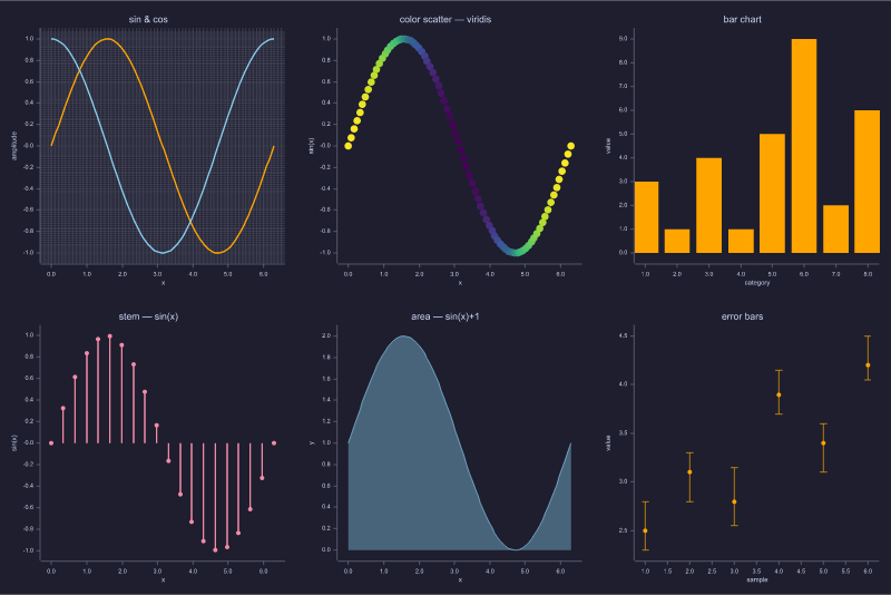
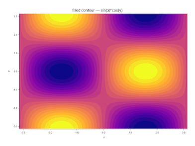
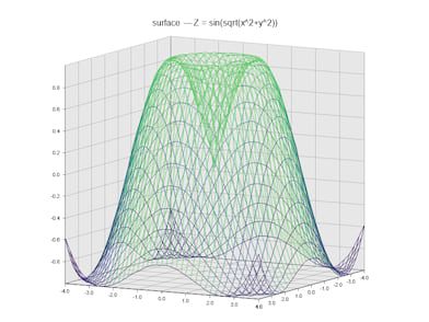
Chart types
| Call | Requires | Description |
|---|---|---|
plot(y) / plot(x, y) |
plot |
ASCII line chart; x inferred when omitted |
plot(x, M) |
plot / plot-svg |
Multi-series: each row of M is one series |
scatter(x, y) |
plot |
ASCII point cloud |
bar(y) / bar(x, y) |
plot |
Vertical bar chart; negative bars drop below baseline |
stem(y) / stem(x, y) |
plot |
Discrete-sequence: line from y=0 + tip marker |
stairs(y) / stairs(x, y) |
plot |
Piecewise-constant step function |
hist(v) |
— | Histogram to terminal (Sturges default bins) |
hist(v, n) |
— | Histogram with n uniform bins |
hist(v, edges) |
— | Histogram with caller-supplied edge vector |
loglog(x, y) |
plot |
Log₁₀ on both axes |
semilogx(x, y) |
plot |
Log₁₀ x-axis, linear y |
semilogy(x, y) |
plot |
Linear x-axis, log₁₀ y |
plot3(x, y, z) |
plot |
3D line; ASCII uses orthographic projection |
scatter3(x, y, z) |
plot |
3D point cloud; ASCII uses orthographic projection |
fill(x, y) / fill(x, y, style) |
plot |
Filled polygon; ASCII uses ░ density grid, file uses Polygon element |
area(x, y) / area(x, y, style) |
plot |
Filled area under curve (closes polygon to y=0 baseline) |
polar(theta, r) |
plot |
Polar chart — coordinate transform then render_line_xy |
quiver(x, y, u, v) |
plot |
Vector field: Unicode arrows (ASCII) / shaft+arrowhead polygons (SVG/PNG) |
text(x, y, 'label') |
plot |
Text annotation at data coordinate — flushed with next render |
errorbar(x, y, e) |
plot |
Symmetric error bars; ASCII compact table, SVG/PNG shaft+cap elements |
errorbar(x, y, e_low, e_high) |
plot |
Asymmetric error bars with independent lower/upper extents |
scatter(x, y, sz, c) |
plot |
Per-point color scatter: c drives colormap lookup; sz scalar or vector |
pie(v) |
plot |
Pie chart; ASCII bar-art table, SVG/PNG wedge polygons |
pie(v, labels) |
plot |
Pie chart with explicit slice labels (cell array) |
pie(v, explode, labels, 'f.svg') |
plot-svg |
Pie with explode offsets, labels, and file export |
yyaxis('left') / yyaxis('right') |
plot |
Switch active Y axis; subsequent plot/ylabel/ylim apply to that axis |
clabel() |
plot |
Enable level labels on the next contour/contourf render (ASCII: footer line; SVG/PNG: inline text per isoline) |
imagesc(Z) |
plot |
False-colour heat-map of matrix Z (ASCII density chars) |
imagesc(Z, 'f.svg') |
plot-svg |
False-colour image saved to SVG/PNG (800 × 600 px) |
imagesc(Z, 'f.png', W, H) |
plot-svg |
False-colour image at custom W × H pixels |
Style strings and colors
Color specification forms (accepted by all styled plot functions):
| Form | Example | Description |
|---|---|---|
| Single-letter | 'r', 'b' |
MATLAB-compatible short code |
| Full name | 'red', 'orange', 'purple', 'gray' |
Full English name |
Hex #RRGGBB |
'#FF4400' |
24-bit hex color |
| 1×3 RGB matrix | [1 0.27 0] |
Values in [0, 1] |
'color', value |
'color', 'red' |
Named arg for bar/stem/hist/quiver |
An optional style string argument (before the file path) sets color, marker, and line style for plot, scatter, fill, area — MATLAB-compatible:
| Code | Color | Code | Line style | Code | Marker |
|---|---|---|---|---|---|
r |
red | - |
solid | . |
point |
g |
green | -- |
dashed | o |
circle |
b |
blue | -. |
dash-dot | x |
cross |
c |
cyan | : |
dotted | + |
plus |
m |
magenta | * |
star | ||
y |
yellow | s |
square | ||
k |
black | d |
diamond | ||
w |
white | ^ |
triangle |
plot(x, y, 'r--')                % red dashed line
plot(x, y, 'orange')             % full color name
plot(x, y, '#1A6ECC')            % hex color
plot(x, y, [0.8 0.2 0.1])        % RGB matrix
bar([1 3 2 5], 'color', 'purple')  % 'color' named arg
hist(v, 20, 'color', '#FF8800')    % hex via named arg
Style strings affect SVG/PNG output only; ASCII charts are always monochrome.
Append a file path to save instead of print to terminal:
| Call | Requires | Description |
|---|---|---|
plot(x, y, 'f.svg') |
plot-svg |
SVG vector graphic (800 × 600) |
plot(x, y, 'f.png') |
plot-svg |
PNG raster image (800 × 600) |
plot(x, y, 'ascii') |
plot |
Force ASCII even when plot-svg is active |
hist(v, 20, 'h.svg') |
plot-svg |
Histogram saved to file |
plot3(x, y, z, 'f.svg') |
plot-svg |
3D line to file (SVG or PNG) |
scatter3(x, y, z, 'f.png') |
plot-svg |
3D scatter to file |
colormap('viridis') |
— | Named colormap for next imagesc (viridis/inferno/magma/plasma/hot/cool/jet/gray) |
colormap(M) |
— | Custom colormap from N×3 matrix (values in [0, 1]) |
colorbar() |
— | Append colour-scale legend strip to next file export |
subplot(rows, cols, k) |
— | Activate panel k in a rows×cols grid; enters accumulating mode |
hold('on') / hold('off') |
— | Overlay multiple series; hold('off') flushes to ASCII (no subplot) |
savefig('f.svg') |
plot-svg |
Commit last panel and write composed figure to SVG/PNG |
Annotations
Set annotations before the render call — they are consumed and cleared by the next render:
| Function | Effect |
|---|---|
title('text') |
Chart title |
xlabel('text') / ylabel('text') / zlabel('text') |
Axis labels (zlabel used by plot3/scatter3) |
xlim([lo, hi]) / ylim([lo, hi]) / zlim([lo, hi]) |
Override axis range |
legend(s1, s2, …) |
Series labels for multi-series SVG/PNG charts |
grid / grid('on') / grid('off') |
Toggle grid (SVG/PNG only; default off) |
theme('light'|'dark') |
Colour theme — 'dark' uses Catppuccin Mocha palette (SVG/PNG) |
bgcolor(color) |
Override figure background color (beats theme) |
fontsize(n) |
Override title and axis-label font size in pixels |
linewidth(f) |
Override default line stroke width for all series |
markersize(n) |
Override default marker radius for all series |
gridcolor(color) |
Override grid line color (requires grid('on')) |
gridwidth(n) |
Override grid line stroke width (requires grid('on')) |
axis('equal'|'tight'|'off'|'on') |
Axis scale mode: equal px/unit, no margin, hidden, or default |
x = linspace(0, 2*pi, 80);

% ASCII line chart
title('sin(x)')
xlabel('x (radians)')
plot(x, sin(x))

% Multi-series SVG with legend and grid
M = [sin(x); cos(x)];
legend('sin', 'cos')
grid('on')
plot(x, M, 'trig.svg')

% Dark theme with custom line width
theme('dark')
linewidth(2)
plot(x, sin(x), 'sin_dark.svg')

% Equal-scale axes (circles appear as circles)
t = linspace(0, 2*pi, 120);
axis('equal')
plot(cos(t), sin(t), 'circle.svg')

% Histogram with explicit edges
hist(randn(1, 500), -3:0.5:3, 'dist.png')

% 3D helix to SVG
t2 = linspace(0, 4*pi, 120);
title('3D helix')
zlabel('z = t/(4π)')
plot3(cos(t2), sin(t2), t2/(4*pi), 'helix.svg')
See examples/plot_demo.calc (ASCII), examples/plot_file/plot_file.calc (file export),
examples/plot_extended.calc (bar/stem/stairs/hist/loglog),
examples/plot3_demo.calc (3D ASCII), examples/plot3_file/plot3_file.calc (3D file export),
examples/colormap/imagesc_demo.calc (imagesc/colormap heat-maps),
examples/subplot_demo/subplot_demo.calc (2×2 subplot grid),
examples/hold_demo/hold_demo.calc (hold on/off overlay),
examples/color_system_demo/color_system_demo.calc (unified color system), and
examples/figure_appearance_demo/figure_appearance_demo.calc (figure appearance — Phase 30.6)
for full worked examples. Run help plot in the REPL for a quick reference.
Bitwise Functions
All require non-negative integer arguments — combine naturally with 0xFF, 0b1010, 0o17 literals.
| Function | Description |
|---|---|
bitand(a, b) |
Bitwise AND |
bitor(a, b) |
Bitwise OR |
bitxor(a, b) |
Bitwise XOR |
bitshift(a, n) |
Left shift (n > 0) / logical right shift (n < 0) |
bitnot(a) |
NOT within 32-bit window |
bitnot(a, bits) |
NOT within bits-wide window (1–53) |
[ 0 ]: bitand(0xFF, 0x0F)
[ 15 ]: bitxor(0xFF, 0x0F)
[ 240 ]: bitshift(1, 8)
[ 256 ]: bitnot(5, 8)
[ 250 ]:
Comparison & Logical Operators
Comparison operators return 1 (true) or 0 (false):
| Operator | Meaning |
|---|---|
== |
Equal |
~= or != |
Not equal |
< |
Less than |
> |
Greater than |
<= |
Less or equal |
>= |
Greater or equal |
Logical operators:
| Operator | Meaning |
|---|---|
~expr or !expr |
Logical NOT (unary) |
&& |
Logical AND |
|| |
Logical OR |
! and != are C/shell-style aliases for ~ and ~=.
Precedence (low → high): || → && → comparisons → : → +/- → *// → ^ → unary (-, ~) → primary
[ 0 ]: 3 > 2
[ 1 ]:

[ 0 ]: 3 == 3
[ 1 ]:

[ 0 ]: 5 ~= 5
[ 0 ]:

[ 0 ]: ~0
[ 1 ]:

[ 0 ]: 2 > 1 && 3 > 2
[ 1 ]:
Element-wise on matrices — comparisons produce a 0/1 mask of the same shape:
[ 0 ]: v = [1 2 3 4 5];
[ 0 ]: v > 3
ans =
   0   0   0   1   1

[ [1×5] ]: v .* (v > 3)    % zero out elements <= 3
ans =
   0   0   0   4   5
Strings
ccalc supports two string types, matching MATLAB/Octave:
Char arrays — single quotes
[ 0 ]: greeting = 'Hello!'
greeting = Hello!
[ 'Hello!' ]: length(greeting)
[ 6 ]:
Char arrays are numeric-compatible — arithmetic converts each character to its ASCII code:
[ 0 ]: 'a' + 0        % ASCII of 'a'
[ 97 ]:
[ 0 ]: 'abc' + 1      % shift each code by 1
ans =
   98   99   100
String objects — double quotes
[ 0 ]: s = "Hello"
s = Hello
[ '"Hello"' ]: s + ", World!"
[ '"Hello, World!"' ]:
String objects use + for concatenation.
String built-ins
| Function | Description |
|---|---|
num2str(x) / num2str(x, N) |
Number → char array (N digits) |
str2num(s) |
Char array → number (error on failure) |
str2double(s) |
Char array → number (NaN on failure) |
strcat(a, b, ...) |
Concatenate strings |
strcmp(a, b) |
Case-sensitive equality → 0/1 |
strcmpi(a, b) |
Case-insensitive equality → 0/1 |
lower(s) / upper(s) |
Case conversion |
strtrim(s) |
Strip leading/trailing whitespace |
strrep(s, old, new) |
Find-and-replace |
sprintf(fmt, v1, ...) |
Format string (C printf), returns char array |
ischar(s) |
1 if char array, else 0 |
isstring(s) |
1 if string object, else 0 |
length(s), numel(s), and size(s) all work on strings.
Datetime & Duration
UTC datetime and duration values are first-class types. Timestamps are stored as seconds since the Unix epoch (1970-01-01 00:00:00 UTC).
Constructors
datetime('2024-06-01')                      % from ISO 8601 date string
datetime('2024-06-01 09:30:00')             % date + time
datetime(2024, 6, 1)                        % from year, month, day
datetime(2024, 6, 1, 9, 30, 0)             % from six components
datetime(ts, 'ConvertFrom', 'posixtime')    % from Unix timestamp

duration(1, 30, 0)    % 1 h 30 min → Duration
hours(2)              % 2 hours
minutes(90)           % 90 minutes
seconds(45)           % 45 seconds
days(1)               % 1 day
milliseconds(500)     % 500 ms
years(1)              % 365.2425 days
NaT is the Not-a-Time constant (analogous to NaN for numbers). Durations display as HH:MM:SS.
Arithmetic
| Expression | Result |
|---|---|
datetime + duration |
DateTime |
datetime - duration |
DateTime |
datetime - datetime |
Duration |
duration + duration |
Duration |
duration * scalar |
Duration |
t  = datetime(2024, 1, 1);
t2 = t + hours(3);           % 2024-01-01 03:00:00
elapsed = t2 - t;            % Duration: 03:00:00
fprintf('%g minutes\n', minutes(elapsed))   % 180
Component and duration extractors
year(dt)   month(dt)   day(dt)    % DateTime → Scalar
hour(dt)   minute(dt)  second(dt)

hours(d)   minutes(d)  seconds(d)  days(d)  milliseconds(d)  % Duration → Scalar
Predicates
isdatetime(x)   % 1 if DateTime or DateTimeArray
isduration(x)   % 1 if Duration or DurationArray
isnat(x)        % 1 if NaT; 0 for any other value
Formatting
datestr(dt)                     % '15-Jun-2024 09:30:00'
datestr(dt, 'yyyy/MM/dd')       % custom pattern
datevec(dt)                     % [y m d H M S] row vector
datenum(dt)                     % MATLAB serial date number
posixtime(dt)                   % Unix timestamp as scalar
fprintf('%s\n', dt)             % ISO: '2024-06-01 09:30:00'
fprintf('%s\n', dur)            % HH:MM:SS: '01:30:00'
Array operations
% Matrix literals produce DateTimeArray / DurationArray
dates = [datetime(2024,1,1); datetime(2024,2,1); datetime(2024,3,1)];
durs  = [hours(1); hours(2); hours(3)];

% diff — successive differences
d = diff(dates);    % DurationArray  (each element = next − prev)
fprintf('%g days\n', days(d))
Complex Numbers
i and j are pre-set to the imaginary unit 0 + 1i. Complex numbers
work with the same operators and functions as real numbers:
[ 0 ]: 3 + 4*i
[ 3 + 4i ]: abs(ans)
[ 5 ]: angle(3 + 4*i) * 180/pi
[ 53.1301023542 ]:
Create, decompose, and manipulate:
z = complex(3, 4)    % 3 + 4i
real(z)              % 3
imag(z)              % 4
conj(z)              % 3 - 4i
z'                   % 3 - 4i  (conjugate transpose)
isreal(z)            % 0
Arithmetic works for all combinations of complex and real scalars:
(3 + 4*i) * (1 - 2*i)   % 11 - 2i
i^2                       % -1    (exact integer exponentiation)
i^4                       %  1
Complex built-ins
| Function | Description |
|---|---|
real(z) |
Real part (real(5) → 5) |
imag(z) |
Imaginary part (imag(5) → 0) |
abs(z) |
Modulus sqrt(re²+im²) |
angle(z) |
Argument atan2(im, re), radians |
conj(z) |
Complex conjugate re - im*i |
complex(re, im) |
Construct from two real scalars |
isreal(z) |
1 if im == 0, else 0 |
Complex matrices
Any matrix literal with at least one complex element becomes a ComplexMatrix.
Real elements are promoted automatically. Full arithmetic, Hermitian transpose
(A'), plain transpose (A.'), element-wise built-ins (real, imag,
abs, conj, angle, isreal), and reductions (trace, diag, sum,
prod, mean) all work on ComplexMatrix.
A = [1+2i, 3-4i; 5, 6+1i]    % 2×2 ComplexMatrix
A'                              % conjugate transpose
abs(A)                          % real Matrix of element-wise moduli
trace(A)                        % Complex scalar (sum of diagonal)

% Indexed assignment: real Matrix auto-upcasts to ComplexMatrix
B = zeros(3, 3)
B(2, 2) = 1 + 2i               % B is now ComplexMatrix
eig(A) returns a ComplexMatrix column vector when a real non-symmetric
matrix has complex conjugate eigenvalue pairs, enabling stability analysis:
d = eig([0, 1; -4, -1.2])      % ComplexMatrix [complex pair]
fprintf('stable: %d\n', all(real(d) < 0))
Since Phase 27, fft() returns a ComplexMatrix instead of a Cell array.
Access bins with X(k) and get the magnitude spectrum with abs(X).
See examples/complex_matrix.m, examples/complex_matrix_ext.m, and help complex for more details.
Formatted Output
fprintf — print to stdout
fprintf(fmt, v1, v2, ...) prints formatted output using C-style conversion specifiers:
| Specifier | Meaning |
|---|---|
%d, %i |
Integer (truncated to whole number) |
%f |
Fixed-point decimal |
%e |
Scientific notation (1.23e+04) |
%g |
Shorter of %f and %e |
%s |
String (char array or string object) |
%% |
Literal % |
Width, precision, and alignment flags follow standard C printf conventions:
fprintf('%8.3f\n', pi)      %     3.142
fprintf('%-10s|\n', 'hi')   % hi        |
fprintf('%+.4e\n', 1000)    % +1.0000e+03
fprintf('%05d\n', 42)       % 00042
Escape sequences: \n (newline), \t (tab), \\ (backslash).
When there are more arguments than conversion specifiers, the format string repeats (Octave behaviour):
fprintf('%d ', 1, 2, 3) % 1 2 3
sprintf — format to string
Same as fprintf but returns the result as a char array instead of printing:
label = sprintf('R = %.1f Ohm', R);
disp(label)
File I/O
File handles
fd = fopen('log.txt', 'w');         % open for writing; returns fd (≥3) or -1 on failure
fprintf(fd, 'x = %.4f\n', x);      % write formatted text to file
fclose(fd);                         % close; returns 0 or -1

fd = fopen('data.txt', 'r');        % open for reading
line = fgetl(fd);                   % read one line, newline stripped; -1 at EOF
raw  = fgets(fd);                   % read one line, newline kept
fclose(fd);

fclose('all');                      % close all open file handles
Modes: 'r' read, 'w' write (create/truncate), 'a' append, 'r+' read+write.
File descriptor 1 = stdout, 2 = stderr.
Delimiter-separated data
dlmwrite('results.csv', A);         % write matrix, comma-separated
dlmwrite('results.tsv', A, '\t');   % explicit delimiter

data = dlmread('results.csv');      % read; auto-detect ',' / '\t' / whitespace
data = dlmread('results.tsv', '\t');
CSV tables — readmatrix / readtable / writetable
Higher-level CSV functions with header row support and type inference.
% readmatrix — numeric data, auto-skip non-numeric header
A = readmatrix('sensor.csv')                   % header skipped automatically
A = readmatrix('data.tsv', 'Delimiter', '\t')  % explicit delimiter

% readtable — first row always the header; returns Struct of columns
T = readtable('grades.csv')
scores = T.score      % Matrix N×1  (numeric column)
names  = T.name       % Cell         (string column)

% writetable — write Struct to CSV with header row
T.name  = {'Alice', 'Bob', 'Carol'};
T.score = [91; 85; 78];
writetable(T, 'out.csv')
writetable(T, 'out.tsv', 'Delimiter', '\t')
Column type inference in readtable: if every cell in a column is parseable
as a number (empty cells → NaN), the column becomes a Matrix N×1; otherwise
a Cell of Str. writetable accepts the same column types and applies RFC 4180
quoting automatically for values containing the delimiter or quotes.
Filesystem queries
isfile('data.csv')          % 1 if the path is an existing file, else 0
isfolder('output/')         % 1 if the path is an existing directory, else 0
pwd()                       % current working directory as a char array

exist('x', 'var')           % 1 if variable x is in the workspace
exist('x', 'file')          % 2 if file exists on disk (MATLAB numeric code)
exist('x')                  % checks workspace first, then filesystem
Directory listing
dir returns a struct array; each element has fields name, folder (absolute path), isdir, and bytes.
entries = dir('.')           % list current directory (.  and .. always first)
entries = dir('*.csv')       % glob — only matching files (no . or ..)
entries = dir()              % same as dir('.')

% Walk a directory
for k = 1:numel(entries)
    if ~entries(k).isdir
        fprintf('%s  %d bytes\n', entries(k).name, entries(k).bytes);
    end
end
Non-existent path → empty struct array, no error.
Workspace with explicit path
save                            % save all variables to default path
save('session.mat')             % save all variables to named file
save('session.mat', 'x', 'y')  % save specific variables only
load('session.mat')             % load variables from named file

path = 'session.mat';
save(path)                      % variable reference also accepted
Scalars, char arrays, and string objects are persisted. Matrices, complex values, and functions are always skipped.
JSON
Requires the
jsonfeature flag:cargo build --release --features jsonWithout this flag, calling either built-in returns an informative error. Both names always appear in tab completion.
% Decode — JSON string → ccalc Value
s = jsondecode('{"name":"Alice","scores":[88,92,75]}')
s.name       % → 'Alice'  (Str)
s.scores     % → [88  92  75]  (Matrix 1×3)

jsondecode('[1, 2, 3]')          % → [1  2  3]  (all-numeric → Matrix)
jsondecode('[1, "two", true]')   % → {1, 'two', 1}  (mixed → Cell)
jsondecode('null')               % → NaN
jsondecode('true')               % → 1

% Encode — ccalc Value → compact JSON string
jsonencode(42)                   % → '42.0'
jsonencode('hello')              % → '"hello"'
jsonencode([1 2 3])              % → '[1.0,2.0,3.0]'
jsonencode(s)                    % → '{"name":"Alice","scores":[88.0,92.0,75.0]}'
jsonencode(nan)                  % → 'null'
Type mapping:
JSON → ccalc (jsondecode) |
ccalc → JSON (jsonencode) |
|---|---|
object {…} → Struct |
Struct → object |
all-numeric array → Matrix 1×N |
Matrix 1×N → flat array |
mixed array → Cell |
Matrix M×N → array of row arrays |
string → Str |
Cell → array |
number → Scalar |
Scalar(NaN) → null |
true/false → Scalar (1/0) |
Str/StringObj → string |
null → Scalar(NaN) |
Inf/Complex/Function → error |
Reading a JSON file (combine with fgetl for single-line JSON):
fid = fopen('data.json', 'r');
raw = fgetl(fid);
fclose(fid);
data = jsondecode(raw);
MAT Files
Requires the
matfeature flag:cargo build --release --features matWithout this flag, calling
load('*.mat')returns an informative error.loadalways appears in tab completion.
% Assignment form — returns a Struct of all variables in the file
data = load('results.mat');
data.score        % Scalar
data.readings     % Matrix
data.label        % Str (char array)
data.sensor.gain  % nested Struct field

% Bare form — injects all variables directly into the workspace
load('results.mat')
score             % now a workspace variable
Type mapping:
| MAT type | ccalc value |
|---|---|
double (1×1) |
Scalar |
double (M×N) |
Matrix |
char array |
Str |
struct |
Struct |
| struct array | StructArray |
cell array |
Cell |
| null / empty | Scalar(NaN) |
Backed by matrw = "=0.1.4". Complex and sparse matrices are not yet supported.
Control Flow
Multi-line control flow blocks are supported in both REPL and script mode.
REPL multi-line input
The REPL detects unclosed blocks and buffers lines with a continuation prompt until end is seen. Press Ctrl+C to cancel an incomplete block.
[ 0 ]:   for k = 1:3
  >>   fprintf('%d\n', k)
  >> end
1
2
3
if / elseif / else
score = 73;
if score >= 90
  grade = 'A';
elseif score >= 70
  grade = 'C';
else
  grade = 'F';
end
fprintf('grade: %s\n', grade)
for
Iterates over a range (or matrix columns):
total = 0;
for k = 1:10
  total += k ^ 2;
end
fprintf('sum of squares: %d\n', total)   % 385
while
x = 1.0;
while abs(x ^ 2 - 2) > 1e-12
  x = (x + 2 / x) / 2;
end
fprintf('sqrt(2) ≈ %.15f\n', x)
break and continue
for n = 1:20
  if mod(n, 2) == 0
    continue       % skip even numbers
  end
  if n > 9
    break          % stop after 9
  end
  fprintf('%d ', n)
end
switch / case / otherwise
switch code
  case 200
    msg = 'OK';
  case 404
    msg = 'Not Found';
  otherwise
    msg = 'Unknown';
end
fprintf('%d: %s\n', code, msg)
No fall-through — only the first matching case runs. Works with scalars and strings. otherwise is optional.
do ... until
Octave post-test loop — the body always runs at least once, then the condition is checked:
x = 1;
do
  x *= 2;
until (x > 100)
fprintf('%d\n', x)   % 128
break and continue work inside do...until.
User-defined functions
Named functions use the function ... end block syntax:
function result = factorial_r(n)
  if n <= 1
    result = 1;
    return
  end
  result = n * factorial_r(n - 1);
end

factorial_r(7)   % 5040
Multiple return values are separated with [...]:
function [mn, mx, avg] = stats(v)
  mn  = min(v);
  mx  = max(v);
  avg = mean(v);
end

data = [4 7 2 9 1 5 8];
[lo, hi, mu] = stats(data);   % lo=1  hi=9  mu=5.14...
Use ~ to discard individual outputs:
[~, top, ~] = stats([10 30 20]); % top = 30
nargin — number of arguments actually passed; useful for optional parameters:
function y = power_fn(base, exp)
  if nargin < 2
    exp = 2;
  end
  y = base ^ exp;
end

power_fn(5)     % 25   (default exponent)
power_fn(2, 8)  % 256
Functions are recursive. They see all other Function/Lambda values
defined in the workspace at the time of the call.
Anonymous functions (lambdas)
sq   = @(x) x ^ 2;
hyp  = @(a, b) sqrt(a^2 + b^2);

sq(7)        % 49
hyp(3, 4)    % 5
Lambdas capture the enclosing environment at definition time (lexical closure):
rate = 0.05;
interest = @(p, n) p * (1 + rate) ^ n;
rate = 0.99;                        % does not affect the lambda
interest(1000, 10)                  % 1628.89  (uses captured 5%)
Pass lambdas to named functions (higher-order functions):
function s = midpoint(f, a, b, n)
  h = (b - a) / n;
  s = 0;
  for k = 1:n
    xm = a + (k - 0.5) * h;
    s += f(xm);
  end
  s *= h;
end

midpoint(@(x) x^2, 0, 1, 1000)         % 0.333333
midpoint(@(x) sin(x), 0, pi, 1000)     % 2.000001
Functions can return functions:
function f = make_adder(c)
  f = @(x) x + c;
end

add5 = make_adder(5);
add5(3)            % 8
add5(make_adder(10)(1))  % 16
Structs and Struct Arrays
Scalar structs group named fields of any type. Fields are accessed with . notation; intermediate structs are created automatically on write.
pt.x = 3;
pt.y = 4;
dist = sqrt(pt.x^2 + pt.y^2)    % 5

car.engine.hp = 190;             % nested struct created automatically
car.engine.hp                    % 190

p = struct('name', 'Alice', 'score', 98.5);
p.name                           % Alice
p.score                          % 98.5
Struct arrays store collections of records. Use indexed assignment to create or grow the array:
pts(1).x = 1;  pts(1).y = 0;
pts(2).x = 3;  pts(2).y = 4;
pts(3).x = 0;  pts(3).y = 5;

numel(pts)   % 3
pts(2).x     % 3

xs = pts.x   % [1 3 0]  — field collection across all elements
ys = pts.y   % [0 4 5]
Dynamic field access — field name computed at runtime:
fname = 'x';
s.(fname)             % read: equivalent to s.x
s.(fname) = 99;       % write: equivalent to s.x = 99

% loop over field names:
fields = {'min', 'max', 'mean'};
for k = 1:numel(fields)
  fprintf('%s = %g\n', fields{k}, stats.(fields{k}))
end
Struct utilities:
fieldnames(s)         % cell array of field names (insertion order)
isfield(s, 'x')       % 1 if field exists, else 0
rmfield(s, 'x')       % copy of s without field 'x'
isstruct(v)           % 1 if v is a struct or struct array, else 0
Structs are displayed MATLAB-style:
s =

  scalar structure containing the fields:

    x: 3
    y: 4

pts =

  1×3 struct array with fields:
    x
    y
Nested or complex fields show compact inline: [1×1 struct], [1×3 double].
Cell Arrays
Cell arrays are heterogeneous 1-D containers where each element can be any value — scalar, matrix, string, or function handle.
c = {42, 'hello', [1 2 3]};   % cell literal
c{1}                           % 42   (brace indexing, 1-based)
c{2}                           % hello
c{3}                           % [1×3 double]
c{4} = 'new';                  % auto-grows beyond current size

iscell(c)                      % 1
numel(c)                       % 4
cell(5)                        % pre-allocated 1×5 cell of zeros
varargin / varargout — variadic functions:
function s = sum_all(varargin)
  s = 0;
  for k = 1:numel(varargin)
    s += varargin{k};
  end
end

sum_all(1, 2, 3)    % 6
sum_all(10, 20)     % 30
cellfun / arrayfun — apply a function to each element:
cellfun(@sqrt, {1, 4, 9})          % [1  2  3]
cellfun(@(x) x*2, {1, 4, 9})       % [2  8  18]
arrayfun(@(x) x^2, [1 2 3 4])      % [1  4  9  16]
@funcname handles — wrap any builtin or named function as a callable:
f = @sqrt;   f(16)            % 4
g = @abs;    g(-7.5)          % 7.5
containers.Map
A string-keyed associative array (lookup table). Equivalent to Python's dict.
% Construct from key/value cell arrays
prices = containers.Map({'apple', 'banana', 'cherry'}, {1.5, 0.75, 2.0});

prices('apple')           % 1.5  — read by key
prices('date') = 3.5;     % insert new key
prices('banana') = 0.99;  % update existing key
prices.Count              % 4    — number of entries

isKey(prices, 'apple')    % 1
isKey(prices, 'mango')    % 0

k = keys(prices)          % {'apple', 'banana', 'cherry', 'date'}  (sorted)
v = values(prices)        % {1.5, 0.99, 2.0, 3.5}  (same order as keys)

remove(prices, 'date');   % remove in-place
prices.Count              % 3
Maps are not saved by ws/save (same policy as matrices and cells).
help map for the full reference.
case {v1, v2} in switch — matches if the switch expression equals any element:
switch x
  case {1, 2, 3}
    disp('small')
  otherwise
    disp('not small')
end
run() / source()
Execute a script file in the current workspace. Variables defined in the script persist in the caller's scope (MATLAB run semantics):
a = 252; b = 105;
run('euclid_helper')      % looks for euclid_helper.calc, then .m
fprintf('gcd = %d\n', g)  % g was set by the helper

source('utils')           % Octave alias for run()
Extension resolution for bare names: .calc is tried first (native), then .m (compatibility).
Search path (addpath / rmpath / path / genpath)
A session search path controls where run() looks for scripts. Entries are checked after the current working directory:
addpath('/my/scripts')            % prepend — highest priority
addpath('/my/utils', '-end')      % append  — lowest priority
rmpath('/my/scripts')             % remove entry
path()                            % display current path
addpath(genpath('/my/libs'))      % add /my/libs and all its subdirectories
genpath(dir) returns dir and all its subdirectories as a path-separator-delimited string (; on Windows, : on Unix).
Persistent paths can be configured in ~/.config/ccalc/config.toml:
path = [
  "~/.config/ccalc/lib",    # exact directory only
  "/home/user/scripts/",    # trailing slash → dir + all subdirectories
]
Error Handling
Scripts can raise, catch, and recover from runtime errors without crashing the session.
% Raise an error with a formatted message
error('value must be positive, got %g', x)

% Print a warning and continue
warning('result may be inaccurate')

% try/catch — anonymous (swallow error)
try
  x = risky_compute(data)
catch
  x = 0
end

% try/catch — named: e.message holds the error string
try
  result = inv(A) * b
catch e
  fprintf('caught: %s\n', e.message)
  result = zeros(size(b))
end

% Inline fallback — default evaluated only on error
n = try(str2num(s), 0)          % 0 if s is not a valid number

% Protected call — returns [ok, value_or_message]
[ok, x] = pcall(@inv, A)
if ~ok
  fprintf('inv failed: %s\n', x)
end

% Last error message
lasterr()                        % message from most recent error
lasterr('')                      % clear
Compound assignment operators
| Operator | Meaning |
|---|---|
x += e |
x = x + e |
x -= e |
x = x - e |
x *= e |
x = x * e |
x /= e |
x = x / e |
x++ |
x = x + 1 |
x-- |
x = x - 1 |
++x |
x = x + 1 |
--x |
x = x - 1 |
All forms desugar at parse time — no performance penalty.
REPL commands
| Command | Action |
|---|---|
exit, quit |
Quit |
cls |
Clear the screen |
help, ? |
Show cheatsheet |
help <topic> |
Detailed help (see below) |
who |
List all defined variables |
clear |
Clear all variables |
clear <name> |
Clear a single variable |
format |
Reset to short (5 significant digits) |
format <mode> |
Switch display mode (see below) |
format <N> |
N decimal places (e.g. format 4) |
hex / dec / bin / oct |
Switch display base |
base |
Show ans in all four bases |
ws / save |
Save workspace to disk |
wl / load |
Load workspace from disk |
save('path') |
Save to explicit file |
save('path', 'x', 'y') |
Save specific variables |
load('path') |
Load from explicit file |
config |
Show config file path and active settings |
config reload |
Re-read config.toml and apply changes |
| Ctrl+C / Ctrl+D | Quit |
Help topics: syntax functions userfuncs cells map structs errors bases vars script format matrices files control datetime setops poly prompt highlight examples
Prompt customization
The prompt is fully customizable via ~/.config/ccalc/config.toml:
[repl]
# Content: {ans} {line} {user} {host} {cwd} {cwd_short} {time}
# Colours: {red} {green} {blue} {cyan} {gray} {reset} {bold} {#RRGGBB} …
prompt1 = "{gray}({line}){reset} [ {ans} ]: "
prompt2 = "  >> "
Run config reload to apply changes without restarting. Run help prompt for the full placeholder reference.
Syntax highlighting
The REPL highlights input in real time. Keywords appear in yellow, numbers in cyan, strings in green, comments in dark gray, and built-in function names in bright cyan. Unclosed strings or brackets are shown in red.
Colours can be overridden in config.toml:
[highlight]
enabled  = true         # set to false to disable
# keywords = "yellow"
# numbers  = "cyan"
# strings  = "green"
# comments = "dark_gray"
# builtins = "bright_cyan"
# errors   = "red"
Colour formats: named ("yellow"), 8-bit ("color256(220)"), 24-bit truecolor
("#FFD700"), and "bold:<colour>" for bold rendering. Run help highlight
for the full reference.
Keyboard shortcuts
| Key | Action |
|---|---|
| ↑ / ↓ | Browse input history |
| Ctrl+R | Reverse history search |
| ← / → / Home / End | Cursor movement |
| Ctrl+A | Go to beginning of line |
| Ctrl+E | Go to end of line |
| Ctrl+W | Delete word before cursor |
| Ctrl+U | Delete from cursor to beginning of line |
| Ctrl+K | Delete from cursor to end of line |
| Ctrl+L | Clear screen |
| Ctrl+C / Ctrl+D | Quit |
Number formatting and bases
Display format
The format command controls how numbers are displayed (MATLAB-compatible):
| Command | Mode | Example for pi |
|---|---|---|
format |
short | 3.1416 (5 sig digits, default) |
format short |
short | 3.1416 |
format long |
long | 3.14159265358979 |
format shortE |
shortE | 3.1416e+00 |
format longE |
longE | 3.14159265358979e+00 |
format bank |
bank | 3.14 (2 decimal places) |
format rat |
rat | 355/113 (rational approx) |
format hex |
hex | 400921FB54442D18 (IEEE 754 bits) |
format + |
+ | + (sign only) |
format compact |
— | suppress blank lines |
format loose |
— | add blank line after outputs |
format N |
custom | format 4 → 0.3333 |
format affects disp(), assignment output, and the REPL prompt — not fprintf/sprintf (which use their own specifiers).
See help format for full documentation.
Very large (|n| >= 1e15) and very small numbers switch to scientific notation automatically in short/long modes.
Number bases
Input literals — mix bases freely in any expression:
| Prefix | Base | Example |
|---|---|---|
0x |
hex | 0xFF → 255 |
0b |
binary | 0b1010 → 10 |
0o |
octal | 0o17 → 15 |
Display base — controls how the prompt and results are shown:
| Command | Effect |
|---|---|
hex |
Switch display to hexadecimal |
dec |
Switch display to decimal (default) |
bin |
Switch display to binary |
oct |
Switch display to octal |
base |
Show ans in all four bases |
[ 0 ]: 0xFF + 0b1010
[ 265 ]: hex
[ 0x109 ]: + 0b10
[ 0x10B ]: dec
[ 267 ]:
Inline base suffix — evaluate an expression and switch display base in one step:
[ 0 ]: 0xFF + 0b1010 hex
[ 0x109 ]:
base command:
[ 10 ]: base
2  - 0b1010
8  - 0o12
10 - 10
16 - 0xA
Expression conversion — when the display base is non-decimal and the expression contains literals in other bases, the converted expression is printed before the result:
[ 0x6 ]: 0b11 + 0b11
0x3 + 0x3
[ 0x6 ]:

[ 0b110 ]: 2 + 0b110 + 0xa
0b10 + 0b110 + 0b1010
[ 0b10010 ]:
Examples
Implicit multiplication:
[ 0 ]: 2(3 + 1)
[ 8 ]:

[ 0 ]: (2 + 1)(4 - 1)
[ 9 ]:
Compound interest — 1000 at 7% for 10 years:
[ 0 ]: 1000 * 1.07 ^ 10
[ 1967.15135729 ]:
Pythagorean hypotenuse — sides 3 and 4:
[ 0 ]: sqrt(3^2 + 4^2)
[ 5 ]:
Variables — monthly mortgage:
[ 0 ]: rate = 0.06 / 12
rate = 0.005
[ 0 ]: n = 360
n = 360
[ 0 ]: factor = (1 + rate) ^ n
factor = 10.9357...
[ 0 ]: 200000 * rate * factor / (factor - 1)
[ 1199.1010503 ]:
Angle conversion — degrees to radians, then sine:
[ 0 ]: 30 * pi / 180
[ 0.5235987756 ]: sin()
[ 0.5 ]:
Script files
When reading from a file (ccalc < formula.txt) you have three tools to control output:
Comments
% starts a comment (Octave/MATLAB convention). # is a supported alias (Octave and shell style). Both can appear as the first character on the line (full-line comment) or inline after an expression.
% Cylinder volume: V = pi * r^2 * h
pi * 5^2      % pi * r^2, r = 5

# same as above — hash-style comment
pi * 5^2      # inline hash comment
Semicolon — suppress output
A trailing ; evaluates the expression and updates ans, but prints nothing.
Use it to silence intermediate steps.
rate = 0.06 / 12;     % monthly rate — silent
n = 360;              % 30-year term — silent
factor = (1 + rate) ^ n;
200000 * rate * factor / (factor - 1)
fprintf('Monthly payment ($): ')
disp(ans)
disp(expr) — print value
disp(expr) evaluates the expression and prints the result.
It does not update ans.
disp(ans)             % print current ans
disp(rate * 12)       % print expression result
fprintf — print formatted text
fprintf(fmt, v1, ...) prints formatted output using C-style specifiers.
No newline is added automatically — include \n explicitly.
fprintf('=== Resistors in series ===\n')

R_total = 100 + 220 + 470;
fprintf('Total resistance: %d Ohm\n', R_total)

fprintf('=== Parallel combination ===\n')

R_par = 1 / (1/100 + 1/220);
fprintf('Parallel resistance: %.2f Ohm\n', R_par)
Output:
=== Resistors in series ===
Total resistance: 790 Ohm
=== Parallel combination ===
Parallel resistance: 68.75 Ohm
Example files
The examples/ directory contains annotated formula files ready to run:
| File | Description |
|---|---|
cylinder.calc |
Volume and surface area of a cylinder |
mortgage.calc |
Monthly mortgage payment |
data_storage.calc |
Real GiB capacity of a "500 GB" drive |
resistors.calc |
Series, parallel resistance, voltage divider, power |
ac_impedance.calc |
AC impedance, phase angle, dB level, bit width |
matrix_ops.calc |
Rotation, linear system solve, element-wise ops |
sequences.calc |
Ranges, linspace, indexing, slicing, finite differences |
logic.calc |
Comparison, logical NOT, &&/||, masks, soft clipping |
bitwise.calc |
Bitmask construction, register bit fields, RGB colour packing |
vector_utils.calc |
nan/inf, reductions, sort/find/unique, end indexing, reshape/flip |
complex_numbers.calc |
Complex arithmetic, polar form, built-ins, AC circuit |
strings.calc |
Char arrays, string objects, arithmetic, built-ins, unit labels |
string_regex.calc |
Phase 21: contains/startsWith/endsWith, strjoin, strsplit roundtrip; regexp/regexpi/regexprep log parser — requires --features regex for sections 5–9 |
datetime.calc |
Phase 22: datetime/duration constructors, arithmetic, component extractors, predicates, formatting (datestr/datevec/datenum/posixtime), array operations, project-timeline example |
set_operations.m |
Phase 23: triu/tril, repmat, kron, cross, dot, intersect/union/setdiff/ismember, sub2ind/ind2sub, repelem; voter-overlap analysis example |
polynomials.m |
Phase 24: polyval, polyfit, roots, poly, conv, deconv, interp1; curve fitting and interpolation examples |
fft_demo.calc |
Phase 26: fft, ifft, zero-padded FFT, fftshift/ifftshift, fftfreq, two-tone power spectrum — requires --features fft for fft/ifft |
complex_matrix.m |
Phase 27: complex matrix literals, arithmetic, conjugate transpose, real/imag/abs/conj/angle/isreal, indexing, shape functions, DFT matrix example |
complex_matrix_ext.m |
Phase 27.5: indexed assignment / auto-upcast, block concatenation, trace/diag/sum/prod/mean on ComplexMatrix, complex eigenvalues for stability analysis, polynomial roots via companion matrix |
formatted_output.calc |
fprintf/sprintf specifiers, flags, escape sequences, data table |
format_modes.calc |
All format display modes: short/long/shortE/bank/rat/hex/+/compact |
file_io.calc |
File I/O: fopen/fclose/fgetl/fgets, dlmread/dlmwrite, isfile/isfolder/exist/pwd, save/load with path |
dir_demo\dir_demo.m |
dir() directory listing: plain dir, glob patterns, field access, non-existent path |
csv/csv.calc |
CSV tables: readmatrix (header auto-skip, NaN for empty), readtable (Struct of columns), writetable (RFC 4180 quoting), tab-separated variant |
json/json.calc |
JSON encode/decode: primitives, arrays, objects, nested structs, roundtrip, file I/O, dataset analysis — requires --features json |
control_flow.calc |
Core control flow: if/elseif/else, for, while, break/continue, compound operators; grade classifier, prime sieve, Newton-Raphson, Collatz |
extended_control_flow.calc |
Extended control flow: switch/case, do...until, run()/source(); exit-code classifier, unit converter, digit sum, Euclidean GCD |
user_functions.calc |
User-defined functions and lambdas: recursion, multiple return values, nargin, anonymous functions, lexical capture, midpoint integration, higher-order functions |
cell_arrays.calc |
Cell arrays: literals, brace-indexing, auto-grow, @funcname handles, cellfun/arrayfun, varargin/varargout, case {…}, function pipelines |
structs.calc |
Scalar structs: field assignment/read, nested structs, struct() constructor, fieldnames/isfield/rmfield/isstruct, 3-D vector example |
struct_arrays.calc |
Struct arrays: indexed creation, element access, field collection → matrix/cell, loop building, fieldnames/isfield, nested fields, inventory ledger |
error_handling.calc |
Error handling: error/warning, lasterr, try/catch, try(expr,default), pcall, nested and loop-safe error recovery |
indexed_assignment.calc |
Indexed assignment: element/slice/submatrix write, growing vectors with end+1, cell array growth, logical mask read/write |
plot_demo.calc |
plot/scatter ASCII terminal charts, title/xlabel/ylabel annotations, polynomial-fit visualisation — requires --features plot |
plot_file/plot_file.calc |
plot/scatter to SVG and PNG files, inferred-x form, practical polynomial-fit export — requires --features plot-svg |
plot_extended.calc |
bar, stem, stairs, hist (auto/manual/edge bins), loglog/semilogx/semilogy, multi-series plot(x,M), xlim/ylim/grid — ASCII, requires --features plot |
plot_extended_file/plot_extended_file.calc |
Same chart types saved to SVG/PNG files, multi-series with legend+grid, histogram variants — requires --features plot-svg |
plot3_demo.calc |
plot3/scatter3 3D ASCII plots via orthographic projection — requires --features plot |
plot3_file/plot3_file.calc |
plot3/scatter3 helix, Lissajous, scatter cloud exported to SVG/PNG — requires --features plot-svg |
colormap/imagesc_demo.calc |
imagesc with all 8 colormaps, colorbar, gradient/radial/sine-wave matrices — requires --features plot-svg |
colormap/mandelbrot.calc |
Mandelbrot escape-count heat-map with colormap('inferno') + colorbar — requires --features plot-svg |
colormap/julia.calc |
Julia set with colormap('magma') + colorbar — requires --features plot-svg |
subplot_demo/subplot_demo.calc |
2×2 subplot grid: sin, cos, bar, hist — saved to SVG — requires --features plot-svg |
hold_demo/hold_demo.calc |
Overlaid sin and cos series using hold on/off; ASCII and SVG variants |
fill_area_polar_demo/fill_area_polar_demo.calc |
Phase 30e: fill/area ASCII+SVG, polar circle + rose curve, all 8 style colors, all 4 line styles, color+linestyle combos |
quiver_demo/quiver_demo.calc |
Rotational flow field u = -y, v = x — ASCII Unicode arrows + SVG export |
annotations/annotations.calc |
text() labels placed at data coordinates, flushed with quiver() |
primitives_demo/primitives_demo.calc |
Phase 32a: line, patch, rectangle in standalone and hold mode |
errorbar_demo/errorbar_demo.calc |
Phase 32b: symmetric + asymmetric errorbar, hold-mode overlay with plot |
scatter_color_demo/scatter_color_demo.calc |
Phase 32b: per-point color scatter(x,y,sz,c) with viridis/jet colormaps and hold mode |
pie_demo/pie_demo.calc |
Phase 32c: pie chart with explicit labels, explode offsets, and SVG file export |
yyaxis_demo/yyaxis_demo.calc |
Phase 32d: dual Y-axis chart — temperature vs humidity (ASCII + SVG), population vs growth rate (SVG) |
contour_demo/contour_demo.calc |
Phase 32e: contour, contourf, and clabel() level labels on Gaussian bell + saddle surface |
matrix_newline_demo.m |
Phase 33b: bare newlines as row separators inside [...] — 2D matrices, column vectors, comments on rows, line continuation |
ccalc < examples/mortgage.calc
Building and testing
cargo build            # debug build
cargo build --release  # optimized build
cargo test             # run all tests
cargo bench            # run Criterion benchmarks (release)
cargo bench --bench engine -- loop_10k   # run one benchmark
Optional features:
cargo build --release --features json         # enable jsondecode / jsonencode (serde_json)
cargo build --release --features fft          # enable fft / ifft (rustfft)
cargo build --release --features plot         # enable ASCII terminal plots (textplots)
cargo build --release --features plot-svg     # enable SVG + PNG file export (plotters)
cargo build --release --features plot-all     # both plot tiers
cargo build --release --features blas         # link system OpenBLAS — faster A*B, inv, \, svd, …
cargo build --release --features blas-static  # same, but statically linked (no runtime dep)
cargo build --release --features json,fft,plot-all  # combine features
BLAS accelerates all matrix multiply and solve operations (pure-Rust is
used by default and is sufficient for matrices up to ~200×200).
Requires libopenblas-dev on Linux or brew install openblas on macOS.
The API is identical in both builds.
Project structure
crates/
  ccalc/src/
    main.rs           — entry point, mode detection (arg / pipe / REPL), CLI flags
    repl.rs           — REPL loop, run_pipe(), run_expr(), shared evaluate() core
    help.rs           — help text
  ccalc-engine/src/
    lib.rs            — crate root, public module exports
    env.rs            — Value enum, Env type (HashMap<String, Value>), workspace save/load
    eval.rs           — AST types (Expr, Op), evaluator, formatters, Base/FormatMode, built-ins
    exec.rs           — block executor: exec_stmts(), Signal enum, call_user_function(),
                        BODY_CHUNK_CACHE (compiled function-body cache)
    io.rs             — IoContext — file descriptor table for fopen/fgetl/fprintf/etc.
    parser.rs         — tokenizer + recursive-descent parser, Stmt enum
    vm/
      mod.rs          — Opcode enum, Instr (8-byte fixed), Chunk, IterState, CompileError
      compile.rs      — compile(&[StmtEntry]) → Chunk; is_compilable() pre-scan
      exec.rs         — vm_exec(chunk, env, …) — main bytecode dispatch loop
  ccalc-engine/benches/
    engine.rs         — Criterion benchmark suite (scalar ops, fib, loop, matmul, fn calls, fft)
Cargo.toml            — workspace manifest (single source of truth for version)
CHANGELOG.md          — version history
License
MIT
Dependencies
~3–14MB
~134K SLoC